Home Science Page Data Stream Momentum Directionals Root Beings The Experiment
Potential Impact has been talked about and described in equations, but its fundamentals have been ignored. Let us first define a few symbols.
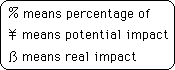
'¥' means potential impact. It is normally followed by two elements, i.e. ¥(x, y). The first element is the part; the second element is the measure, derivative or what-not that the first element is part of. If there is no second element then its existence should be defined by its context. ¥(x, y) means the potential impact of the first element, x, upon the second element, y. 'ß' means real impact. ß (x, y), which uses the same notation as '¥', means the real impact of the first element, x, upon the second element, y. %ß (x, y) means the percentage of the real impact of the first element, x, upon the second element, y. %¥(x, y) means the percentage of the potential impact of the first element, x, upon the second element, y.
'%' means 'percentage of'. Percentage, generally, is defined as the part divided by the whole.
Rephrasing this general statement we could say that the percentage could be defined as the contribution of the part to the whole. This second statement is a little more precise and will avoid ambiguities later on.
The contribution of the part is sometimes much less than the part itself, especially when speaking of measures and derivatives. When speaking of an itinerary, the length of each individual part of the trip is divided by the length of the whole trip to determine its percentage of the whole trip. When speaking of the average amount of miles one traveled each day then one must first know how many days the trip was in addition to the length of the individual part to know the percentage effect of that one day upon the measure miles per day. In this instance it is unnecessary to know the full length of the trip, although it could be easily figured out by multiplying the miles per day by the number of days. The point made is that sometimes a part equals its contribution to the whole, i.e. when the whole is the sum of the parts, and sometimes it doesn't, i.e. when the whole is a composite measure, based upon other arithmetic manipulations other than simple adding.
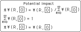
The sum of the potential impacts of all the parts that contribute to the whole is one, one hundred percent. Thus the potential impact of the whole upon itself is always one. This is a truism.
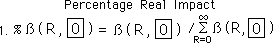
The percentage potential impact of the part upon the whole is equal to the potential impact of the part upon the whole divided by the potential impact of the whole upon itself, by the definition of percentage.
Because the potential impact of the whole upon itself is always one, the percentage potential impact of the part upon the whole is always equal to the potential impact of the part upon the whole. This is stated in the equation below. Henceforth %¥ will not be used because of its redundancy.
In a similar fashion the sum of the real impacts of all the parts that contribute to the whole is equal to the whole. This is also a truism.
The real impact of the part upon the whole is equal to its potential impact upon the whole times itself. Conversely potential impact could be defined as that which would be multiplied times the part to get the real impact of that part upon the whole. With our trip analogy, the real impact of an individual day upon the miles per day would be simply the number of miles traveled that day divided by the number of days. Hence the potential impact of that day upon the miles per day would be 1 divided by the number of days. Each of the days of the trip would have the same potential impact upon the miles per day. But depending upon the amount of miles traveled each day, the real impact of each day upon the whole miles per day measure would be different, because the size of each part could be quite different.
The percentage of the real impact of the part upon the whole would be equal to the real impact of the part upon the whole divided by the real impact of the whole upon itself, by definition of percentage.
The real impact of the whole measure upon itself is the whole measure, Equation. 5. Also the real impact of the part upon the whole is equal to the potential impact of the part times the part itself, Equation. 6. Substituting these facts into equation 7, we find that the percentage of the real impact of the part upon the whole is equal to the ratio of the part to the whole times the potential impact of the part. If the whole is equal to one then the percentage real impact of the part equals the real impact of the part. Otherwise the real impact of the part is not equal to the percentage real impact as it was with the potential impact.
Potential & Real impact measures have no meaning in traditional studies because they are so fixed and boring. For the Mean Average the potential impact of each of the elements that makes up the average is always the same. It is always the one divided by the number of elements, N, going into the average. (Note that X-bar has no subscript. This indicates that it is a Mean Average, not a Decaying Average.) The real impact is the element divided by the number of elements. The percentage real impact is the ratio of the piece to the average divided by N, the number of elements in the average. With traditional averages each part has an equal potential contribution to the whole hence their potential impacts are equal. There is no need to examine this boring phenomenon.

The potential impact of the parts upon the averages of continuous functions is even more bizarre. Because the whole is something while the parts of continuous functions are infinitesimals, the potential impact of each of the individual parts is zero. With an infinite summation these infinitesimals add up to the whole, as they should, but their individual potential impact is equal to zero. Because the real impact and the percentage of the real impact both contain the potential impact in their computation, they both equal zero also. Boy, these are fascinating results! They show why there has been such interest in potential impact over the ages. Ha! Ha! Joke.
Decaying Averages and their derivatives have been ignored over the ages by most scientists, because of their worship of the god of predictable functions. As mentioned in other notebooks, many scientists still believe that everything can be reduced to natural law, God's laws. Unpredictability and spontaneity are not a characteristic of the universe under this view. Ultimately every phenomenon can be reduced to a function, perhaps a complicated function but a function, nevertheless. Those that believe in the god of functions either ignore spontaneity as a characteristic of existence or label those who believe in spontaneity as superstitious, primitive, backwards, unscientific, illogical or emotional.
Decay itself tends to be avoided as a phenomenon because of a bad press. Most often decay is related to continuous functions, which can only be calculated with the assistance of tables or computers. No mortal man could ever be expected to calculate natural logarithms in his head. Hence decay has been elevated to a divine status, which only the priests of science and industry and their tools can deal with. Quite the opposite is true.
In our notebooks we have shown that a contextual approach to data collection and their measures have built decay into the system in such an easy way that every one, even cave men and women and animals, use decaying averages regularly to compute the realm of probability, which facilitates survival. It turns out that decaying averages are much easier to compute than traditional averages and much more useful immediately. They are sensitive and relevant. Because of the widespread use of decaying averages, contrary to the image given by the popular press, we have focused much attention upon these derivatives. One of the interesting features of the decaying averages and their derivatives is the potential impact of the parts. Because of decay each of the parts has a different potential impact upon the whole. Following is a look into potential impact.
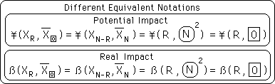
Each member of a Data Stream has a unique potential impact upon The Decaying Average and its Derivatives. This justifies the study. First look at the bubble below to review notation. The elements of each equality are just different ways of writing the same thing. It is not new information, just new ways of expressing potential and real impact. We will use the last style, the number-square, because of its simplicity.
The percentage potential impact of any element on the Decaying Average would be the potential impact of that element divided by the sum of the potential impact of all the elements making up the Decaying Average. The total potential impact on any derivative is always one. Hence the percentage potential impact is the same as the potential impact for the Decaying Average. This only confirms the results derived above. However it reveals a way of checking potential impact. If the sum of all the potential impacts does not equal one then something is wrong. Perhaps not all the impacts are included or maybe the formula for potential impact is wrong.
The percentage real impact of any data point upon the Decaying Average would be given by the ratio of the real impact of that one data point divided by the sum of all the real impacts. This is by the definition of percentages.
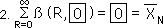
The sum of all the real impacts upon the measure is the measure itself – in this case the Decaying Average.
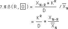
Substituting, the percent real impact of a data point on the Decaying Average would be the real impact of the data divided by the Decaying Average. This is the same result as above in a more specific setting.
The real impact of the data point is the product of the data point, itself, and its potential impact. This again by definition. The second line is identical to the first except written in circle terminology for clarification.
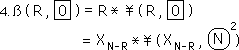
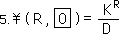
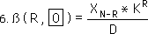
The potential impact of any Data point upon the Decaying Average is given by the formula below. It is a function of R, the number of separations from Now. The impact of the data point is scaled R times and divided by D once because the potential impact of the data points has only been spread over one dimension for the Decaying Average.
The real impact of the data point is the product of the potential impact and the data point, substitution and definition.
Substituting we find that the percentage real impact is equal to the potential impact times the ratio of the part and whole. This is as was expected and so confirms our previous derivation.
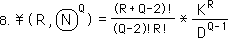
In the Raveled Numbers Notebook we established that the following is the equation for potential impact of any data point on any multiple raveling.
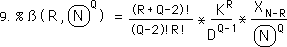
Multiplying this by the ratio of the part to the whole yields the percentage of real impact of the data point upon the raveling.
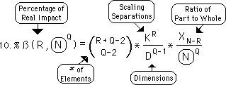
Rewriting the first element as a combination we see the different parts of the equation for the percentage of real impact of a data point on a Raveled Number.
Because it helps us lead into our next topic, we will point out that with each additional raveling that the potential impact of the Data Point is spread across another dimension. Hence its impact is divided by D, the Decay Factor, for each new dimension that the its potential impact is spread over.